Releases
2.2.1
About
The difference with respect to version 2.2.0 is that this version can be installed via Anaconda or pip.
Installation
Install via Anaconda:
conda install -c WilcoTerink SPHY=2.2.1
or install via pip:
pip install SPHY==2.2.1
2.2.0
About
Background
Glaciers in previous SPHY model releases were not mass conserving; i.e. they were implemented as a fixed mass generating glacier melt using a degree day factor. This means that:
- Rainfall on the glacier was not accounted for, and needs to be corrected for as a pre-processing step
- Snowfall, accumulation of snow, and snow melt on glacier grid cells was not taken into account
- Redistribution of ice from the accumulation to the ablation zone was not simulated; i.e. the dynamic retreat or advance of glaciers could not be simulated
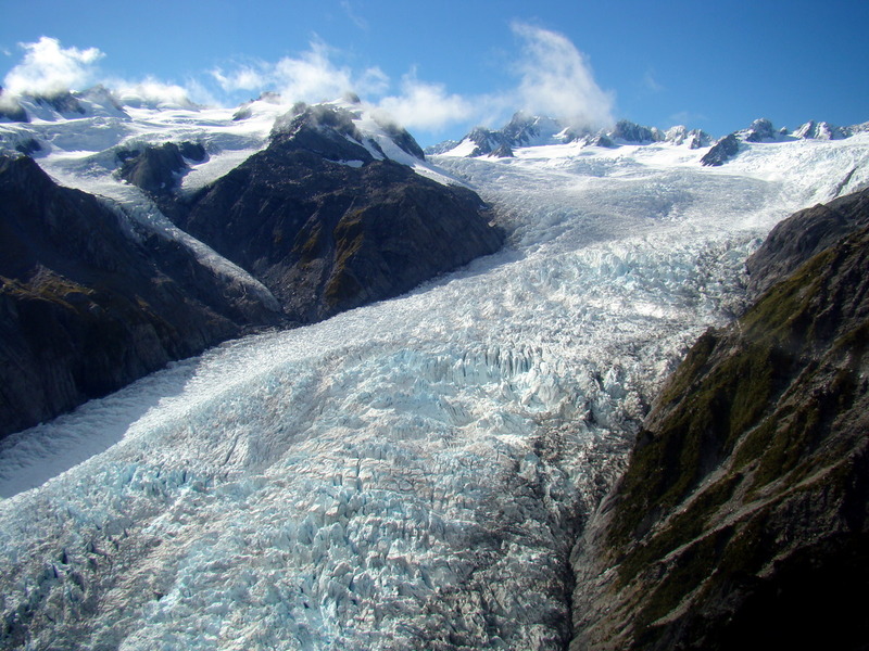
Figure 20 A glacier in New Zealand.
Several methods exist to model glacier dynamics. E.g., [Bahr1997] performed a scaling analysis of the mass and momentum conservation equations and showed that glacier volumes can be related by a power law to more easily observed glacier surface areas. The disadvantage of this approach is that it is a lumped method and can therefore not be applied on a gridded surface. Another method is described by [Huss2010], who uses a \(\Delta\) h-parameterization to describe the spatial distribution of the glacier surface elevation change in response to a change in mass balance. It is an empirical glacier-specific function derived from observations in the past that can easily be applied to large samples of glaciers. However, a disadvantage of this methodology is that a large number of observations (multiple DEMs of the same glacier) from the past is required. [Weertman1957] and [Immerzeel2012b] described another method, known as Weertman sliding [Weertman1957]. The disavantage of this method is that it is only feasible at high spatial model resolutions (<100 m), and it ignores viscous deformation. A good overview of the methods that are available for estimating ice volumes is well-described in [6].
Improved glacier module
The improved glacier module accounts for rainfall and snowfall onto the glacier, accumulation and melt of snow, and redistribution of ice from the accumulation to the ablation zone. These modifications allow glaciers to retreat over time if the melt rate is higher than the accumulation rate. The only data required for the improved module is:
- A high-resolution DEM (higher resolution than the spatial resolution of your model)
- A shapefile with the outlines of the glaciers within your area of interest. The Randolph Glacier Inventory (RGI) is a recommended source for this
- A classification of which areas are debris-free and which are debris-covered
The new module uses the strength of combining PCRaster operations with NumPy and pandas dataframe functionalities. Instead of specifying the spatial distribution of glaciers on a PCRaster model grid, the glacier characteristics are now specified in a csv-file, and the glacier model grids are the initialized from this csv-file. Each line in the csv-file describes the glacier properties for a UID, which is a unique combination of model cell ID, glacier ID, glacier elevation, and a boolean describing if that UID is clean ice or debris-covered. The contents of this csv-file and the creation thereof are described in here.
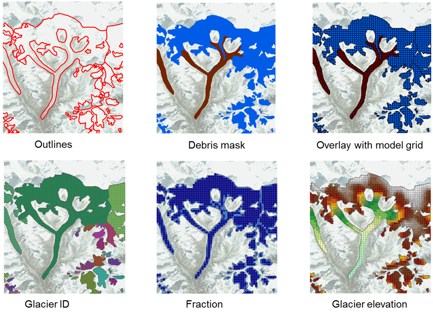
Figure 21 Illustration of steps to prepare input for the improved glacier module.
The new module basically comes down to overlaying your model grid with a higher resolution DEM to allow for the differentation of multiple glacier fractions and associated elevations within one model grid cell. A more accurate represenation of multiple glacier elevations within one model grid cell allows for a more accurate calculation of temperature, and thus melting rates. The more accurate temperature is calculated by lapsing the temperature from the model cell elevation to the elevation of the glacier fraction within that model grid cell. Snow and rain on the glacier are now accounted for, and melt rates adapt based on the presence of a dynamic snow pack; snow is melted before the glacier start melting.
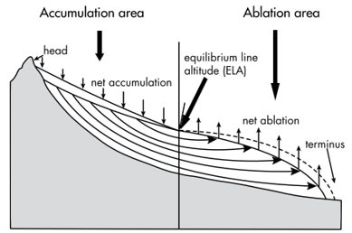
Figure 22 The Equilibrium Line Altitude (ELA), accumulation area, and ablation area of a glacier.
Although the movement of glaciers is a continuous process, modelling this on a daily time-step is not feasible given the level of detailed geophysical information required for this. Glacier movement is the result of ice-redistribution. This is modelled by calculating the difference between the accumulation of snow and the melting of glacier ice on an annual basis (end of the hydrological year). Glaciers have an Equilibrium Line Altitude (ELA) above which the net accumulation of ice occurs and net melt (ablation) occurs below the ELA (Figure 22). If the annual glacier’s mass balance is negative (more ablation than accumulation), then the accumulated mass (snow in accumulation zone) is redistributed over the ablation UIDs according to the ice volume distribution of the cells in the ablation zone. This process may eventually cause glaciers to disappear if the net ablation in a year is larger than the amount of ice available in the accumulation zone.
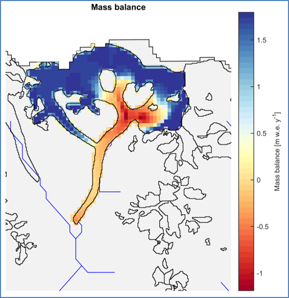
Figure 23 Example of the simulation of the glacier’s average annual mass balance.
Installation
This version can only be installed by downloading it from the SPHY model GitHub repository. A direct link to this release can be found here.
2.1.1
About
The difference with respect to version 2.1.0 is that this version can be installed via Anaconda or pip.
Installation
Install via Anaconda:
conda install -c WilcoTerink SPHY=2.1.1
or install via pip:
pip install SPHY==2.1.1
2.1.0
About
Background
Although most dominant hydrological processes were integrated in previous SPHY release versions, the model was not yet capable of simulating reservoir inflow and outflow. In version 2.1.0, a reservoir module was developed for the SPHY model.
Depending on the availability and quality of reservoir data, the user has two options for simulating reservoir in- and outflow in the SPHY model, being:
The advanced reservoir scheme focuses on a target release, while the simple scheme calculates the outflow based on the actual and maximum reservoir storage. The reservoir schemes can be specified for each individual reservoir, meaning that simple and advanced reservoirs can exist independently from each other. The concepts of these schemes are described in the following two sections.
Simple reservoir scheme
Many studies have implemented reservoir operation schemes into large-scale hydrological models. [Meigh1999] for example used a grid-based model and incorporated reservoir outflow using the following assumptions. For outflow regulation reservoirs, the outflow (Q) was proportional to the current storage (S) raised to the power of 1.5. For water storage reservoirs, any water released was used to meet demands and once the reservoir was filled, the outflow equaled the amount spilled [Hanasaki2006]. A study by [Doll2003] accounted for reservoir flow regulation [Hanasaki2006], and modified the equation of [Meigh1999] to:
with:
This parametrization was developed for global lakes, but is also applied for reservoirs because of a lack of information on their management [Hanasaki2006]. For this reason this reservoir outflow equation was implemented in the SPHY model, and is referred to as the simple reservoir scheme hereafter. The outflow coefficient (k) is generally used as a calibration parameter. An example of the reservoir inflow, outflow and storage is illustrated in Figure 24 for the simple reservoir scheme.
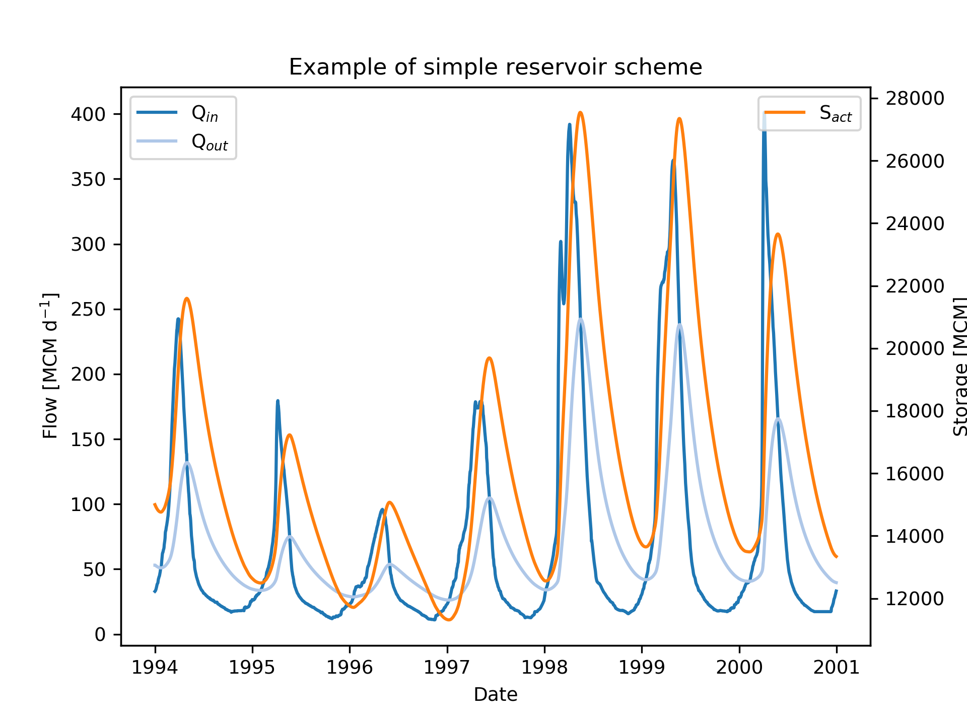
Figure 24 Example of reservoir inflow (Qin), outflow (Qout), and storage (Sact) as modelled by the simple reservoir scheme.
Advanced reservoir scheme
If reservoir management information is available, then it is recommended to use the advanced reservoir scheme. This scheme uses the same approach as is implemented in the SWAT model [Neitsch_2000]. Within the advanced reservoir scheme the user can define a target reservoir release volume, which is season dependent. The user can define two different seasons per year, being a flood and dry season respectively. The target releases that need to be defined are the MAX_FLOW (maximum flow) for the flood season, and the DEM_FLOW (demand flow) for the dry season.
In case of floods it is important to have a large storage capacity available. Therefore, the model tries to release the maximum amount of water from the reservoir during the flood season. The maximum amount of water that can be released depends on the user defined MAX_FLOW, the actual reservoir storage, and the maximum amount of water that is available between the emergency spillway and principal spillway. During the dry season, the model aims to keep the reservoir filled in order to have water available for its water users downstream. During this season, the reservoir outflow depends on the user defined DEM_FLOW (demand flow), the actual reservoir storage, and the maximum amount of water that is available between the emergency spillway and principal spillway. Reservoir outflow for both seasons is thus calculated as:
with:
An example of the reservoir inflow, outflow and storage is illustrated in Figure 25 for the advanced reservoir scheme.
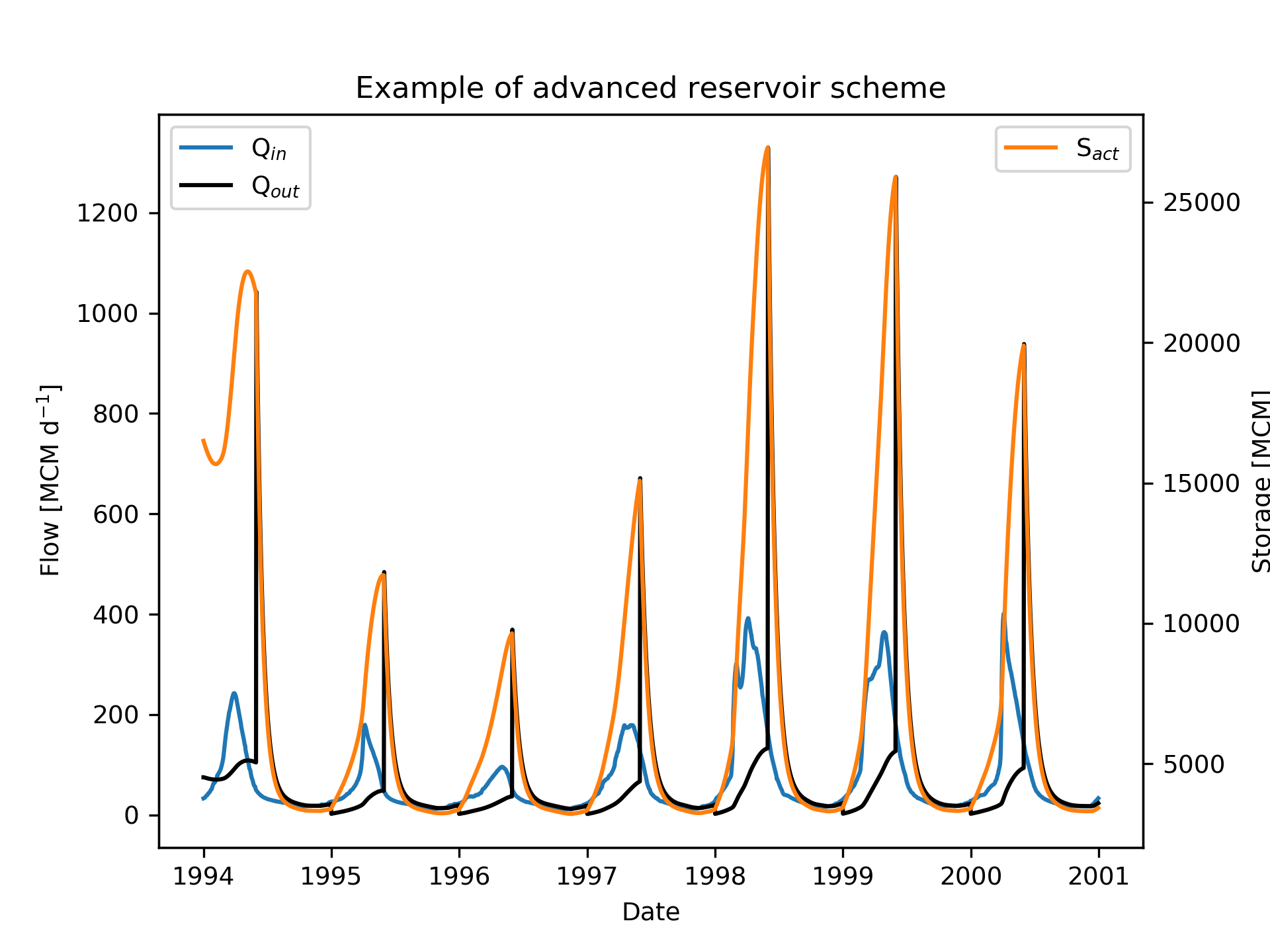
Figure 25 Example of reservoir inflow (Qin), outflow (Qout), and storage (Sact) as modelled by the advanced reservoir scheme. In this example the flood season starts the first of June, and ends by the end of December.
Installation
This version can only be installed by downloading it from the SPHY model GitHub repository. A direct link to this release can be found here.
2.0.4
About
The difference with respect to version 2.0.3 is that this version can be installed via Anaconda or pip.
Installation
Install via Anaconda:
conda install -c WilcoTerink SPHY=2.0.4
or install via pip:
pip install SPHY==2.0.4
2.0.3
About
Bug fix in the reporting function and in the calculation of snow storage and melt water stored in snow pack.
Installation
This version can only be installed by downloading it from the SPHY model GitHub repository. A direct link to this release can be found here.
2.0.2
About
Fixed critical error in the calculation of lateral flow. Lateral flow was originally calculated as:
\(\left(rootlat + rootdrain\right) \cdot \left(1-exp^\frac{-1}{rootTT}\right)\)
This resulted in a continuous outflow of lateral flow with small values for \(rootTT\), even if there was no lateral flow generated in the current timestep. This equation has been fixed to:
\(rootlat \cdot \left(1-exp^\frac{-1}{rootTT}\right) + rootdrain \cdot exp\frac{-1}{rootTT}\)
Installation
This version can only be installed by downloading it from the SPHY model GitHub repository. A direct link to this release can be found here.
2.0.1
About
There was an error in the calculation of the fractional rain. In version 2.0.0 the fractional rain was calculated by multiplying the rain with the rain fraction. This has been fixed by multiplying the rain with \(\left(1-glacfrac\right)\).
Installation
This version can only be installed by downloading it from the SPHY model GitHub repository. A direct link to this release can be found here.
2.0.0
About
SPHY version 2.0.0 [31] is the first offical release of the SPHY model, and was published in Geoscientific Model Development. All model concepts and processes are described in this PDF.
Installation
This version can only be installed by downloading it from the SPHY model GitHub repository. A direct link to this release can be found here.